


1.1 Classifiers
Many classification tools such as the support vector machines, logistic regression, decision trees and feed-forward networks have been successful in modelling but have not had much success in modelling the time dimension of data. Some of these algorithms have adopted the moving window techniques in order to model time.
The disadvantage with these algorithms in modelling time is making the assumption that time has connections independently to the model inputs, therefore fail to capture long-range time dependencies. For example for moving window techniques failing to capture larger effects than the window itself.
1.2 RNNs
RNNs are just like any other feed-forward nets but their major difference is that they are focused on modelling time-steps. It processes the sequences by looping through the elements and maintaining the information relative to the state to what it has seen so far. The simple fact that RNN models the data by creating cycles in the network makes it recurrent in nature.
The availability of looping in connections allows the Recurrent Neural Networks to model time-stamped behaviour such as language, test and time-series datasets. The RNN is trained to compute patterns such that the output at each time, t, is based on both the current input and the inputs on all previous times.
1.2.1 Inputs
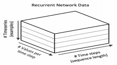
The input data for modelling is more multi-dimensional, the inputs contain three dimensions: the mini-batch size, number of columns in the vector at any epoch and number of epochs.
1.2.2 Vanishing Gradients
RNNs have the problem of vanishing gradient, when the gradient become too large or too small such that it becomes too hard to keep track or retain information about the inputs that have had epochs before. The models of Long Short Term Memory (LSTM) and the Gated Recurrent Unit (GRU) are designed to be able to solve these problems.
1.2.3 LSTM
Includes the memory cell and the gates. Contents of the memory cell are modulated by the input gates and forget gates. Gating allows retaining of information over deeper time epochs hence allowing the LSTM model to overcome the vanishing gradient problem.
Properties of LSTM: Better equations update
Better backpropagations
Each LSTM unit, which is the same as the artificial, neuron has connections from the previous epoch and connections from the previous layer. The memory cell thus allows the network to maintain state over the epochs.
Components of LSTM units: The block input
The three gates that is, the input gate, the output gate and the forget gate
Memory cell
Output functions
The peephole connections
1.2.4 GRU
The major difference between GRU and LSTM is that GRU fully exposes the memory contents using a leaky integration. It’s simpler to compute and implement.
1.1 TENSORFLOW
Tensorflow is a powerful library suited from machine learning tasks developed by Google and open sourced in November 2015. TensorFlow offers a lot of machine learning features, and in this exercise the Keras layers are exploited for implementing Recurrent Neural Networks (RNN). The architecture of TensorFlow is shown as below:
1.2 RNNs
Recurrent neural networks are designed to be able to learn from sequential data. The architecture is made in such a way that it is supposed to perform the same task for every object without forgetting the previous. An example is predicting the next word in a sentence which starts with the word that came before that word and using the current word to predict the next word. Generally, any data with time steps or intervals.
The RNN is implemented by the Keras layer. There are largely three implementations such as the SimpleRNN, the LSTM and the GRU. The SimpleRNN is a very simple implementation of an RNN. Therefore, for real world applications, the other two are more useful. The main reason why the SimpleRNN is unusable in large applications is because it is hard for it to learn to keep information about inputs in large time steps. This is known as the vanishing gradient problem. The same problem is encountered by the feed-forward networks, they are many layers deep that it becomes almost impossible to achieve training. This is where the LSTM and the GRU layers come in. (Systems, 2019)
1.2.1 LSTM
Known as the Long Short-Term Memory, was developed in 1997. It’s onto the SimpleRNN, a way to carry information across many time steps. The major component of the LSTM is the memory cell and the gates that is, the forget gate and the input gate. This gating structure allows information to be retained across multiple time-series and hence overcomes the vanishing gradient problem. The LSTM networks contain many LSTM cells and perform well during the learning process.
The memory is the central concept such that it allows the network to maintain the state over time. The main body of LSTM unit is known as the LSTM block.
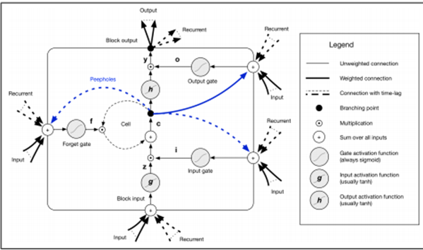
Within the block, there are three gates which have to learn to protect the linear unit from misleading signals, these are; the input gates which protect the unit from irrelevant events, the forget gate that helps the unit forget the previous memory cells and the output gate which exposes the contents of the output of the LSTM unit.
A basic LSTM layer takes input vector x and gives output y. The output is influenced by the input and the history of all the inputs before it. LSTM networks are supervised learning mechanisms which update the weights in the network. The input vectors are trained at one time step in a series of vectors. For each of the sequences of the input vectors, the errors equals the sum of the deviations of all target signals computed by the network. (Patterson & Gibson, 2017)
1.2.2 GRU
The Gated Recurrent Units work much as same as the LSTM, only that they do not use a memory unit to control the flow of information. They can make use of the hidden layers directly without any control. They also have fewer parameters, therefore, the training process is faster. In comparison to LSTM, they might have a lower expressiveness with large data. They are made of two gates, the reset gate and the update gate. The reset gate determines how to combine new inputs. The update gate determines how the new input is combined to previous memory. (Chollet, 2018)