


Volatility and Risk – Exploring and Contrasting the Effectiveness of VIX Futures as a Diversification Tool in Equity Portfolios
Abstract
We assess the effectiveness of CBOE volatility index (VIX) based futures index and related Exchange-traded products in reducing downside risk and providing tail risk protection to predominantly equity portfolios. Our analysis shows that around 20% and 10% allocation of VIX medium term futures to an equity and bond-equity portfolio respectively, would have benefited investors looking to reduce downside risks and left tail risks in their portfolios. We also find that equity portfolios with similar allocations towards fixed income or Gold ETPs, have somewhat inferior downside risk and tail risk measures when compared with allocations in VIX medium term futures.
Keywords: Equity Portfolio Management, Asset Allocation, Tail Risk Management, Diversification, CBOE volatility index (VIX), EURO STOXX 50 Volatility (VSTOXX), Performance measurement.
- Introduction
Diversification with negatively correlated or uncorrelated asset classes has been called the “Holy Grail of Investing”1. This is especially true for equities which tend to experience large drawdowns during market risk off events. The positive correlation between traditional asset classes (except maybe bonds) and equities during drawdowns is well documented. Szado (2009) shows the conditional correlation between S&P 500 and almost all major asset classes (including commodities) increased during the 2008-09 Global Financial Crisis (GFC). While US treasury bonds have had a negative correlation with equity returns during crisis periods post 2000, as noted by Harvey et. al. (2019), this is a more recent phenomena in a period characterized by extreme monetary easing and generally supportive background for treasury bonds.
Gold is probably the oldest and the original safe haven asset. Being a real asset, it is considered hedge against long-term inflation, and currency devaluation (especially in emerging/frontier markets). However, Erb & Harvey (2013) cast doubts on Gold as an inflation or even as a tail risk hedge. The authors find that real price of Gold could be a better indicator of its future returns.
There are a number of downside protection strategies like constant proportion of portfolio insurance (CPPI), timeseries momentum, volatility targeting, long put/put spread, short credit risk etc. This study focuses on testing efficacy of long volatility position for tail risk protection in predominantly equity portfolios. This study tries to compare and contrast the diversification and tail risk protection ability of long volatility position with Gold. The long volatility position is expressed through ETPs or indexes based on VIX based futures.
1.1 Volatility as an asset class
The COVID pandemic which impacted the global markets this year has again turned the spotlight on volatility. With the increasing occurrence of left-tail risk events, defined as where the VIX closes up by more than five standard deviations in one day, from once every two years to twice every year after 2008, a 4x increase, it is becoming a significant concern for investors to focus on reducing left-tail risks.
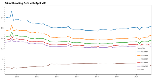
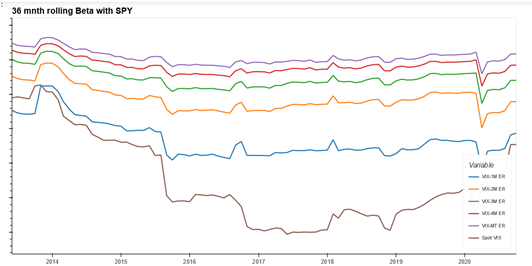
Due to its mean reverting nature, a long volatility position has zero or negative risk premium. However, the fact that the returns from long volatility position are positively skewed and negatively correlated to equities means that volatility products are suggested as diversification tools, allowing liquid long volatility strategies to act as natural shock absorbers by reducing beta to equity markets. Historic rolling correlation and beta of VIX and SPY (iShares S&P 500 ETF; representing the equity position) with other traditional asset classes as well as rolled VIX futures index variants of different maturities can be found in Appendix 4 and 5. The asymmetric nature of negative relationship between VIX/long volatility position and equity returns has been documented in Whaley (2009) and Szado (2009). This means that returns of VIX and VIX based products increase in order of magnitude during an equity market downturn compared to corresponding move when equity returns are positive. We are able to validate this asymmetric relationship for VIX and various VIX/VSTOXX based futures indexes in Appendix 3.
1.2 VIX and VIX based futures
The Chicago Board Options Exchange (CBOE) introduced a Volatility Index (VIX) in 1993 to measure the expected 30-day volatility of the market at-the-money Standard & Poor’s 100 index options. Its popularity grew with time to become the leading indicator of U.S. stock market’s volatility. A decade later, Goldman Sachs and CBOE revised the index to measure volatility in the stock market by basing the index on the Standard & Poor’s 500 index options (SPX), the main index in the U.S. stock market. The new formula calculates VIX as the weighted implied volatility of S&P 500 out of the money (OTM) puts and calls with approximately 30 days to maturity.
But the VIX, being a calculated index value itself, is not directly investable. However, exchange-traded VIX futures contract was introduced in 2004 and VIX options in 2006, both on CBOE. VIX ETPs were launched based on static or dynamic allocation to VIX futures and options were launched in 2009 further opening up investor access to “pure” volatility products. Exchange traded instruments like VIX futures, options and ETF/ETNs tracking them offer transparent, liquid and convenient way to access returns from market volatility (D’Anne, 2012). Where possible, VIX ETPs (or the underlying index) based on constant maturity VIX/VSTOXX rolled futures index especially the 1- month short term rolled futures index and medium term rolled futures index have been used as proxies to represent long volatility position.
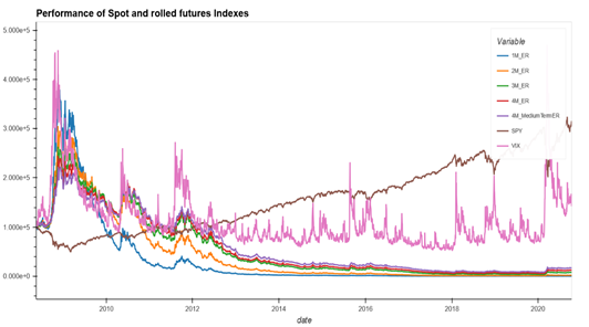
Returns from holding futures position, can be approximately decomposed into spot, roll and collateral return (Ilanmen, 2011). However, for rolled VIX futures indexes and ETPs, roll returns are most significant driver of overall returns. Due to the mean reverting nature, the term structure of VIX futures is upward sloping (or contango) in normal market conditions. Hence, investors in VIX futures contracts incur ongoing costs in the rolling their position which can be a significant drag on performance. This is evident in the performance chart of various rolled VIX futures indexes in Appendix 1. During major market downturns when spot VIX spike, the term structure can become inverted (or in backwardation) driving positive roll returns. This is illustrated in Appendix 2. Due to performance drag from roll costs, standalone exposure to these instruments is not appropriate for long term investors. Our analysis therefore focuses on improvement in risk-adjusted returns and tail risk protection of predominantly equity portfolios, in investors allocate a relatively small portion (<30%) to ETPs or indexes based on rolled VIX futures.
Investing in VIX futures is an indirect way to gain exposure to VIX (D’Anne, 2020). The various VIX futures indexes as well as ETPs differ in terms of their product structure, maturity and roll costs and hence can be significantly different in terms of correlation and beta to spot VIX or equity returns as can be seen in Appendix 4 and 5. Indeed, as we move to longer maturity contracts further out in the term structure, both the correlation and beta to spot VIX decreases, with attendant decrease in roll costs too. We discuss the trade-off between roll costs and beta to spot VIX and equity returns in more detail in the methodology section.
We work with ETPs or indexes based on constant maturity rolled futures position. This allows us to look at the performance while controlling for maturity. We have not considered leveraged, inverse or dynamic VIX based indexes or ETPs in our analysis.
As an aside, long puts can provide tail risk protection too. However, decision needs to be taken on choice of strike price and maturity. Moreover, rolling the long-put position incurs time decay as well roll costs. Similarly, there are other instruments to go long volatility like variance swaps, dynamic replication of straddle/strangle, VIX options etc.
- Literature Review
Szado, (2019) while noting that the VIX index is negatively correlated to equity markets and that the VIX future and options can provide diversification benefits to equity portfolios, found that the upward sloping characteristics of VIX futures reduces portfolio performance and posits that in particular periods, risk-averse investors can find meaningful portfolio diversification benefits with small allocations to long VIX futures and options though there could be significant tax on the portfolio return if investors make large allocations over a long time of flat to bull markets.
Both Deng et al. (2012) and Hill (2013) find that short term VIX future indexes experience larger negative roll yields and may not offer better portfolio diversification than fixed income in a traditional 60/40 equity-bond portfolio. Both also suggested that indexes tracking VIX futures with longer tenors like the medium-term VIX futures index might offer diversification. Gantenbein et. al. (2013) come to a similar conclusion and find that a 10% allocation to the rolled medium term futures index or straightforward dynamic allocation strategy is beneficial for equity portfolios.
According to Alexander et al (2016), the benefits of volatility diversification are never realized despite the frequent perception of the optimality, ex ante, of this diversification. They noted that the benefits are eroded by the high roll costs coupled with the transaction costs and that the exchange-traded volatility only proved to be effective for diversification during the banking crisis of 2008. They further argue that long equity and bond portfolios that were diversified with volatility futures underperformed similar portfolios without diversification or those diversified with other commodities.
A study by Paoloni, (2016) on diversification using VIX options found that a VIX call buying strategy, which was relatively cheap, not only offer sufficient protection during tail risk events but can also indicate when the hedge is not needed.
Berkowitz et al (2018) found that the current VIX related products, in addition to being costly to implement, results in abnormal negative returns. They also found that among all the volatility assets, VIX futures offer the best risk-adjusted return. Nevertheless, this finding obviously goes against the theory that holding VIX should prove beneficial to a portfolio and the findings of Paoloni (2016).
Another study by Shahzad et al (2017), coming across the interesting finding that the performance of assets changes depending on whether there is a crisis or not and thus there is no hedge asset that is absolutely suitable at all market conditions.
Bahaji & Aberkane (2016) notes that the inclusion of VIX futures in a portfolio of assets, VIX futures provided an improved performance over commodities and hedge funds but may yield utility that is below expectation for certain investors.
- Methodology
3.1 Data
As a starting point to our analysis, we extract VIX futures contract prices from CBOE website2. This dataset starts from 2004. Using the daily contract settlement prices, we calculate the constant maturity VIX futures indexes per the details mentioned in the next section. Our constant maturity index calculations are based on the S&P VIX futures index methodology on which popular short term VIX futures ETNs and ETFs are based. Calculating the constant VIX futures index levels ourselves allows going back further in history. We were able to calculate historical index levels starting from November, 2006 for 1-, 2-, 3- and 4-month constant maturity VIX futures index and from May, 2008 for the Medium term VIX futures index. VIX spot index levels were directly downloaded from CBOE’s website (with history based on current methodology starting from 1989).
Similarly, both spot VSTOXX as well as the corresponding 1-month short term and medium-term constant maturity VSTOXX futures index, were directly downloaded from STOXX website3.
All calculated VIX rolled futures index levels (and the corresponding VSTOXX future indexes) are excess return (ER) variants, i.e. they assume that the positions in underlying futures contracts are not collateralized. The difference from total return variants is relatively minor in that the collateral yield from investing on short-term risk-free instruments is not considered.
One of the objectives of our analysis is to simulate historical performance with ETPs accessible to investors as much as possible. We use underlying indexes in case a long enough history of ETF is not available (see Figure 1 for details on indexes and ETPs used to represent various asset classes). To avoid drawing optimistically biased conclusions, we deduct a flat “investor fees” of 85 bps per year from the performance of calculated VIX (and downloaded VSTOXX) rolled futures index levels. This “investor fees” roughly corresponds to the expense ratio we have observed for various VIX/VSTOXX ETPs.
Proshares launched ETP products tracking S&P VIX short term (ticker: VIXY) and medium-term ER indexes (ticker: VIXM) in 2011. We use calculated levels for 1M and medium term VIX futures index adjusted for the above mentioned “investor fees” from 2008 till 2011, and corresponding Proshares ETFs from 2011 onwards. This allows us to look at realized performance of VIX based products across a 12-year span from November, 2008 (i.e. covering most of the GFC period) to October, 2020.
Investing in ETPs also carries other trading costs (bid-ask spreads, commissions, taxes etc.) as well as other costs like redemption fees which we have not factored in our analysis. Wherever possible though we have tried to choose large liquid ETPs with significant tied AUM and long enough performance history which are broadly representative of the underlying asset classes in their respective regions.
Daily adjusted closing prices of all other equity, fixed income and Gold indexes and ETFs are downloaded from yahoo finance. Cash returns are proxied by 1M Libor4 and 1M Euribor5 for US and Europe simulations respectively.
3.2 Calculation of Constant Maturity VIX Futures Index
3.2.1. VIX Short term futures Index calculation: To calculate the daily return of a rolling long position in both the current futures contract and the next Futures contract, the formula (1) is used.
(1)
where
is the corresponding excess return of constant maturity VIX futures Index with maturity i
ERt is the daily excess return,
and which itself is calculated using (2)
(2)
where
is the closing price of the ith month futures (earlier expiring) on day t,
is the closing price of the jth month futures (later expiring) on day t,
and wtj are given by (3) and (4)
(3)
(4)
where
dt is the number of remaining days to expiration,
Tt is the total number of days of the Futures contract from its starting date to its expiration date.
3.2.2. VIX Medium term futures Index calculation: Similarly, the S&P 500 VIX Mid-Term Futures Index gives the daily return of a long position in a portfolio consisting of monthly VIX Futures that maintains a weighted average maturity of five months. The underlying contracts consist of four-, five-, six- and seven-month VIX Futures contract. Everyday a corresponding fraction of the fourth months contract is rolled into seventh-month contracts, while maintaining the positions of fifth- and sixth-months contracts unchanged.
Hence the formula for the daily excess returns becomes (5).
(5)
And where the weights wt in (5) add up to 1 (6).
(6)
And the weight of the fifth- and sixth-month always remain equal.
(7)
3.3 Roll cost calculation
Because all VIX futures expires at given dates, if it’s desired to continue to hold a position in such assets beyond these dates as is often the case, we have to regularly roll part of current futures position into the next futures contract.
The cost incurred in rolling from earlier expiring futures to a later expiring futures, the roll cost, is calculated using the formula (8).
(8)
where
t is the day of the trading,
is the roll cost on day t,
is the closing price of the ith month futures (earlier expiring) on day t,
is the closing price of the jth month futures (later expiring) on day t,
is the fraction rolled from the ith month futures to the jth month futures
3.4 Approach
Once we have the VIX futures index levels, we proceed to simulate results with different static allocation combinations of the main equity asset (SPX or STOXX) and cash/fixed income/gold/long volatility position in VIX futures. Finally, we conduct simulations to further check and contrast the diversification potential of Gold and long volatility position in the traditional 60/40 equity-bond portfolio.
All portfolios with static allocation mixes as described in the result section are rebalanced to their target asset allocation scheme at the last trading day of each month.
3.5 Choice of VIX Futures Index
Since the spot VIX index is not directly investable, a natural question arises on which VIX futures index to use to represent the long volatility position. VIX futures index with short terms to maturity have a higher correlation and beta to spot VIX index as shown in Appendix 3. However, shorter term futures contracts also suffer from higher roll costs. We use the ratio of 36 month rolling beta to spot VIX / average roll costs of the specific contracts as the metric to choose the VIX rolled futures index. As can be seen in Table 1 below, the metric is lowest for the VIX medium term rolled futures index. Roll costs calculations follow the methodology as listed in Liu and Dash (2011).
Table 1. 36 month Rolling Beta to Spot VIX/ Average Roll Costs, Average Daily Roll Costs and % of Days when Roll Cost was Incurred
| Rolling 36 month average | Rolling 60 month average | |||||
| VIX futures index | Average rolling beta to SPY/ average daily roll costs | Average rolling beta to spot VIX/ average daily roll costs | Average rolling beta to SPY/ average daily roll costs | Average rolling beta to spot VIX/ average daily roll costs | Average daily roll costs between 2008 to 2020 (in bps) | % of days between 2008 to 2020 when roll cost was incurred (as opposed to roll yield) |
| VIX-1M* | -16.8% | 2.6% | -16.5% | 2.4% | 23.0 | 80.8% |
| VIX-2M | -19.0% | 2.9% | -17.0% | 2.4% | 13.6 | 78.9% |
| VIX-3M | -24.3% | 3.8% | -19.4% | 2.7% | 8.9 | 78.0% |
| VIX-4M | -26.2% | 4.0% | -19.6% | 2.7% | 7.4 | 76.6% |
| VIX-MT^ | -30.2% | 5.0% | -20.7% | 2.8% | 6.2 | 78.1% |
* VIX- 1M denotes VIX 1-month constant maturity index and similarly for other maturities
^ VIX-MT denotes VIX medium term index
Analysis period Nov’08- Oct’20
Due to the mean reverting nature of volatility, a long volatility position has a zero or negative risk premium. Also, as already discussed, returns from a long volatility position is negatively correlated to equity returns. The asymmetric nature of the negative correlation relationship is reflected in the positive skewness of the return distribution, as can be seen in the historical simulation as shown in Table 2 below.
Spot VIX index is not directly investable and does not incur roll costs, leading to positive returns in the Table 2. Further, as already pointed out, one can also observe that VIX has the highest risk, with volatility declining for rolled futures indexes of longer maturity. All the variants exhibit positive skewness in the return distribution (which as discussed is an important feature of long volatility position).
The VIX medium term indexes incur the lowest rolling costs (have lowest negative returns compared to other VIX futures variants). This further confirms our choice for medium term futures as the instrument of choice to represent the long volatility position.
Table 2. Performance Indicators of Spot and Rolled Futures Indices
| Nov’08 – Oct’20 | Spot VIX | VIX-1M ER | VIX-2M ER | VIX-3M ER | VIX-4M ER | VIX-MT ER |
| Annualized CAGR(%)6 | 2.9 | -45.1 | -29.4 | -20.0 | -16.8 | -14.4 |
| Annualized Arithmetic mean(%) | 36.5 | -35.2 | -20.1 | -12.3 | -10.9 | -9.8 |
| Risk (%) | 91.1 | 75.2 | 58.4 | 48.2 | 41.6 | 36.0 |
| Downside Risk (%) | 50.6 | 36.5 | 29.0 | 24.4 | 21.6 | 19.2 |
| Return/Risk | 0.03 | -0.6 | -0.5 | -0.41 | -0.4 | -0.4 |
| Monthly Skewness | 1.81 | 2.56 | 2.88 | 2.86 | 2.73 | 2.43 |
| Monthly Kurtosis | 5.7 | 9.4 | 13.7 | 14.3 | 13.7 | 11.1 |
| Sharpe-Ratio7 | 0.03 | -0.61 | -0.51 | -0.42 | -0.42 | -0.41 |
| Sortino-Ratio8 | 0.05 | -1.25 | -1.03 | -0.84 | -0.8 | -0.78 |
| Maximum Drawdown (%)9 | -88.7 | -100.0 | -99.8 | -98.9 | -98.0 | -96.7 |
| Calmar Ratio10 | 0.03 | -0.45 | -0.29 | -0.2 | -0.17 | -0.15 |
| Return/Max Drawdown | 0.03 | -0.45 | -0.29 | -0.2 | -0.17 | -0.15 |
| 5% monthly VaR (%) | -29.9 | -25.2 | -20.8 | -16.8 | -14.9 | -14.3 |
| 5% monthly CVaR (%) | -34.2 | -27.8 | -22.5 | -19.0 | -17.7 | -16.0 |
| CVaR ratio11 | 0.01 | -0.18 | -0.13 | -0.1 | -0.09 | -0.08 |
ER stands for the ‘Excess Return’ variant of the indexes. This is equivalent to realized spot and roll returns with uncollateralized positions in underlying futures contracts
- Results
To check the effectiveness of long volatility position as equity risk diversifier, we test different combinations of allocations towards the VIX medium term index and the S&P 500 index (represented by S&P 500 SPDR ETF, ticker: SPY). The equity allocation is kept above 60% and below 100%, so that equity risk still remains the dominant driver of overall portfolio performance.
Further, we contrast the portfolio performance in terms of risk-adjusted returns, with similar allocation combinations of equity and fixed income (represented by iShares Bloomberg Barclays Aggregate Bond index, ticker: AGG) as well as equity and Gold (represented by SPDR Gold Trust, ticker: GLD) and cash (represented by 1-month US Treasury Bill). The risk-adjusted returns for various allocation combinations are shown in Appendix 6.
Historical simulation of allocation schemes with better risk-adjusted performance as well as drawdowns are shown in Table 3. These results show that a ~20% allocation towards VIX medium term futures index can improve risk-adjusted performance with lower drawdowns. A 40% allocation towards cash (and rest in SPY) performs similarly in terms of risk-adjusted terms. The 40% fixed income allocation scheme outperforms the rest in the simulation period, perhaps aided by the favorable return environment for bonds during the post GFC period, followed by the 30% GLD/70% SPY portfolio. We also look at rolling 3-year and 5-year statistics (with overlapping return periods), to avoid basing our conclusion on only fixed horizon historical simulations.
It is well known that the returns of most asset classes are not normally distributed and that risk-adjusted return metrics like Sharpe ratio consider only the first two moments of returns. Xiong and Idzorek (2018) showed that portfolios with lower standard deviation could be more negatively skewed and exhibit higher kurtosis and hence could have higher “crash”/tail risk. Since we are interested in tail risk protection, we are also looking at other downside and tail risk measures like the downside risk, Maximum drawdown, 5% CVaR. We further evaluate the tradeoff between these downside risk measures and excess returns for various portfolios via their Sortino, Calmar and CVaR ratios.
Looking at these measures we find that the portfolio with a 20% allocation to VIX-MT futures exhibits positive skewness, lowest CVaR, maximum drawdown and downside risk with comparable Sortino, Calmar and CVaR ratios to the 30% GLD and 40% AGG portfolios. Notably, the 20% VIX-MT portfolio also has lower kurtosis compared to the 30% GLD and 40% AGG portfolios.
Table 3. Historical Simulation of Different Allocation Schemes of SPY with VIX Medium Term Futures, Fixed Income, Gold and Cash
| Nov’08 – Oct’20 | SPY | SPY 60%/ Cash 40% | SPY 60%/ AGG 40% | SPY 90%/ GLD 10% | SPY 80%/ GLD 20% | SPY 70%/ GLD 30% | SPY 90%/ VIX-MT ER 10% | SPY 80%/ VIX-MT ER 20% | SPY 70%/ VIX-MT ER 30% |
| Annualized CAGR(%) | 9.8 | 6.4 | 7.9 | 9.7 | 9.5 | 9.3 | 8.2 | 6.4 | 4.3 |
| Annualized Arithmetic mean(%) | 10.7 | 6.6 | 8.1 | 10.3 | 10.0 | 9.7 | 8.6 | 6.6 | 4.5 |
| Risk (%) | 15.8 | 9.5 | 9.7 | 14.5 | 13.4 | 12.7 | 11.9 | 9.0 | 8.1 |
| Downside Risk (%) | 12.2 | 7.3 | 7.5 | 11.1 | 10.1 | 9.4 | 8.7 | 6.2 | 5.1 |
| Return/Risk | 0.62 | 0.67 | 0.82 | 0.67 | 0.71 | 0.73 | 0.69 | 0.71 | 0.53 |
| Monthly Skewness | -0.73 | -0.74 | -0.82 | -0.71 | -0.68 | -0.63 | -0.29 | 0.23 | 0.9 |
| Monthly Kurtosis | 1.48 | 1.48 | 2.13 | 1.93 | 2.48 | 2.99 | 1.14 | 1.66 | 2.7 |
| Sharpe-Ratio | 0.59 | 0.61 | 0.76 | 0.63 | 0.67 | 0.69 | 0.65 | 0.65 | 0.46 |
| Sortino-Ratio | 0.76 | 0.79 | 0.98 | 0.83 | 0.89 | 0.93 | 0.88 | 0.95 | 0.74 |
| Maximum Drawdown (%) | -50.7 | -33.8 | -33.2 | -46.5 | -42.1 | -37.4 | -42.2 | -32.6 | -21.9 |
| Calmar Ratio | 0.19 | 0.19 | 0.24 | 0.21 | 0.23 | 0.25 | 0.2 | 0.2 | 0.2 |
| Return/Max Drawdown | 0.19 | 0.19 | 0.24 | 0.21 | 0.23 | 0.25 | 0.2 | 0.2 | 0.2 |
| 5% monthly VaR (%) | -7.9 | -4.7 | -4.4 | -7.0 | -6.0 | -4.7 | -5.0 | -3.6 | -2.6 |
| 5% monthly CVaR (%) | -10.3 | -6.2 | -6.4 | -9.3 | -8.5 | -7.8 | -7.3 | -5.1 | -3.9 |
| CVaR ratio | 0.07 | 0.08 | 0.09 | 0.08 | 0.08 | 0.09 | 0.08 | 0.09 | 0.08 |
| Rolling Statistics | |||||||||
| Average 36months rolling returns | 13.3 | 8.2 | 9.5 | 12.4 | 11.4 | 10.5 | 9.6 | 5.8 | 2.0 |
| Average 36months rolling risk | 12.7 | 7.6 | 7.6 | 11.6 | 10.8 | 10.3 | 9.3 | 6.8 | 6.3 |
| Average 36months rolling return/risk | 1.13 | 1.15 | 1.32 | 1.13 | 1.10 | 1.03 | 1.08 | 0.85 | 0.25 |
| Average 60months rolling returns | 13.4 | 8.2 | 9.4 | 12.2 | 11.0 | 9.8 | 9.4 | 5.5 | 1.5 |
| Average 60months rolling risk | 12.3 | 7.4 | 7.3 | 11.2 | 10.5 | 10.1 | 9.0 | 6.6 | 6.1 |
| Average 60months rolling return/risk | 1.13 | 1.15 | 1.32 | 1.12 | 1.08 | 0.98 | 1.08 | 0.84 | 0.20 |
Continuing from the previous section, we also check whether a long volatility position enhances risk-adjusted returns and reduces drawdowns in a 60% equity and 40% fixed income portfolio (60/40 portfolio). Further, the same results but for other combinations are shown in Appendix 7. Historical simulation of allocation schemes with the best risk-adjusted performance is shown in Table 4. We find that a 10% allocation to VIX medium term futures index enhances risk-adjusted returns with lower drawdowns, CVaR, downside risk with better skewness and kurtosis, though again allocations schemes with Gold show somewhat comparable performances.
Table 4. Historical Simulation of Different Allocation Schemes
| Nov’08 to Oct’20 | SPY | SPY 60%/ AGG 40% | SPY 60%/ AGG 35%/ GLD 5% | SPY 60%/ AGG 30%/ GLD 10% | SPY 60%/ AGG 20%/ GLD 20% | SPY 60%/ AGG 30%/ VIX-MT 10% | SPY 60%/ AGG 20%/ VIX-MT 20% |
| Annualized CAGR(%) | 9.8 | 7.9 | 8.1 | 8.2 | 8.5 | 6.6 | 5.2 |
| Arithmetic mean(%) | 10.7 | 8.1 | 8.2 | 8.4 | 8.7 | 6.7 | 5.3 |
| Risk (%) | 15.8 | 9.7 | 9.8 | 10.0 | 10.6 | 7.5 | 6.7 |
| Downside Risk (%) | 12.2 | 7.5 | 7.5 | 7.6 | 7.9 | 5.4 | 4.4 |
| Return/Risk | 0.62 | 0.82 | 0.82 | 0.82 | 0.8 | 0.89 | 0.78 |
| Monthly Skewness | -0.73 | -0.82 | -0.79 | -0.76 | -0.69 | -0.12 | 0.47 |
| Monthly Kurtosis | 1.48 | 2.13 | 2.38 | 2.62 | 3.01 | 1.79 | 2.11 |
| Sharpe-Ratio | 0.59 | 0.76 | 0.77 | 0.77 | 0.75 | 0.82 | 0.7 |
| Sortino-Ratio | 0.76 | 0.98 | 1 | 1.01 | 1.01 | 1.14 | 1.06 |
| Maximum Drawdown (%) | -50.7 | -33.2 | -33.1 | -32.9 | -32.7 | -27.7 | -22.0 |
| Calmar Ratio | 0.19 | 0.24 | 0.24 | 0.25 | 0.26 | 0.24 | 0.24 |
| Return/Max Drawdown | 0.19 | 0.24 | 0.24 | 0.25 | 0.26 | 0.24 | 0.24 |
| 5% monthly VaR (%) | -7.9 | -4.4 | -4.3 | -4.3 | -4.2 | -2.4 | -2.1 |
| 5% monthly CVaR (%) | -10.3 | -6.4 | -6.4 | -6.4 | -6.6 | -4.5 | -3.5 |
| CVaR ratio | 0.07 | 0.09 | 0.09 | 0.1 | 0.1 | 0.11 | 0.11 |
| Rolling Statistics | |||||||
| Average 36months rolling returns | 13.3 | 9.5 | 9.5 | 9.5 | 9.5 | 6.7 | 3.9 |
| Average 36months rolling risk | 12.7 | 7.6 | 7.7 | 7.9 | 8.5 | 5.6 | 5.0 |
| Average 36months rolling return/risk | 1.13 | 1.32 | 1.29 | 1.25 | 1.14 | 1.22 | 0.73 |
| Average 60months rolling returns | 13.4 | 9.4 | 9.3 | 9.3 | 9.0 | 6.5 | 3.5 |
| Average 60months rolling risk | 12.3 | 7.3 | 7.5 | 7.6 | 8.2 | 5.4 | 4.8 |
| Average 60months rolling return/risk | 1.13 | 1.32 | 1.29 | 1.24 | 1.11 | 1.21 | 0.7 |
Corresponding results for spot VSTOXX, VSTOXX short term and medium term rolled future indices are summarized in Appendix 8. Results in table 6 are broadly in line with the similar simulations for VIX futures indices. Tables 7 summarizes results with different allocations towards VSTOXX medium term future index and STOXX 50 index and comparison with Gold and fixed income allocations. However, we could only simulate the results over the common return period from June-2017 as the European Gold ETF (Xetra-Gold; ticker: 4GLD) levels are only available as from then. Gold seems to be the clear outperformer but we cannot draw any meaningful conclusion given the rather short analysis and since Gold prices have generally been on an upward trend since 2016. Table 8 shows that a 10% allocation to VSTOXX medium term futures in a bond-equity portfolio does enhance risk-adjusted returns as well as lowers tail-risk and drawdowns.
- Conclusions
Investors’ preferences for different aspects of risk is one of the key drivers of asset allocation decisions. Through historical simulations covering a decade and two NBER defined recessions (GFC and Covid pandemic related downturn), we show that around 20% and 10% allocation of VIX medium term futures to an equity and bond-equity portfolio respectively, would have benefited investors looking to reduce downside risks or left-tail risks in their portfolios. VIX medium term futures index (or ETP) is our instrument of choice to represent the long volatility position as it provides the best exposure to volatility per unit of roll cost. Ease of access to these products though transparent ETPs with sufficiently long history also motivates our choice. We also show that predominantly equity portfolios with the above-mentioned allocations towards VIX medium term futures have lower downside and tail risk measures when compared with equity portfolios with similar allocations towards fixed income or Gold ETPs. We are however unable to draw any similar meaningful conclusion for VSTOXX medium term futures index in Europe due to lack of long enough common performance history.
Appendix 1
Appendix 2
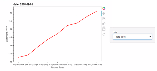
Settlement Price vs Futures Series in Contango
Spot VIX= 76621.16 , SPY =243391.76
Rolling 36-Months Returns: Spot VIX = -0.1357, SPY = 0.1452
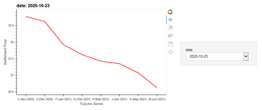
Settlement Price vs Futures Series in Backwardation
(Also serves as an indication that the market is crashing)
Spot VIX= 156712.17 , SPY return=314782.85
Rolling 36-Months Returns: Spot VIX = 0.4049, SPY = 0.1216
Appendix 3
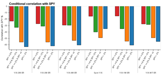
Nov-2008 to Oct-2020
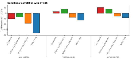
Jan-2011 to Oct-2020
Appendix 4
Appendix 8
Europe results:
Table 6. Performance indicators of spot and rolled futures indices
| Jan’10- Oct’20 | Spot VSTOXX | VSTOXX-1M ER | VSTOXX-MT ER |
| Annualized CAGR(%) | -3.4 | -35.8 | -13.1 |
| Annualized Arithmetic mean(%) | 25.8 | -13.2 | -6.8 |
| Risk (%) | 80.3 | 78.1 | 32.3 |
| Downside Risk (%) | 46.1 | 38.1 | 17.7 |
| Return/Risk | -0.04 | -0.46 | -0.41 |
| Skewness | 2.1 | 2.59 | 2.16 |
| Kurtosis | 10.75 | 10.05 | 9.3 |
| Sharpe-Ratio | -0.04 | -0.46 | -0.4 |
| Sortino-Ratio | -0.07 | -0.94 | -0.74 |
| Maximum Drawdown (%) | -85.5 | -99.7 | -89.1 |
| Calmar Ratio | -0.04 | -0.36 | -0.15 |
| Return/Max Drawdown | -0.04 | -0.36 | -0.15 |
| Rolling Statistics | |||
| Average 36months rolling returns | -3.6 | -37.3 | -17.2 |
| Average 36months rolling risk | 71.0 | 57.1 | 25.5 |
| Average 36months rolling return/risk | -0.07 | -0.7 | -0.71 |
| Average 60months rolling returns | -3.1 | -35.1 | -15.2 |
| Average 60months rolling risk | 72.2 | 56.9 | 25.1 |
| Average 60months rolling return/risk | -0.05 | -0.64 | -0.63 |
Table 7. Performance of Different Allocation Schemes of STOXX 50 Index with VSTOXX Medium Term Futures, Fixed Income, Gold and Cash
| Jun’17 – Oct’20 | STOXX | STOXX 60%/ EAGG 40% | STOXX 80%/ EGLD 20% | STOXX 70%/ EGLD 30% | STOXX 60%/ EGLD 40% | STOXX 90%/ VSTOXX-MT ER 10% | STOXX 80%/ VSTOXX-MT ER 20% | STOXX 70%/ VSTOXX-MT ER 30% | STOXX 60%/ VSTOXX-MT ER 40% |
| Annualized CAGR(%) | -1.52 | 0.57 | 1.6 | 3.13 | 4.64 | 0.13 | 1.52 | 2.66 | 3.56 |
| Arithmetic mean(%) | -0.1 | 1.12 | 2.44 | 3.71 | 4.99 | 0.91 | 1.92 | 2.94 | 3.95 |
| Risk (%) | 16.65 | 10.56 | 13.24 | 11.69 | 10.3 | 12.58 | 9.5 | 8.59 | 10.43 |
| Downside Risk (%) | 13 | 8.4 | 10.25 | 8.96 | 7.76 | 9.18 | 6.31 | 5.48 | 5.8 |
| Return/Risk | -0.09 | 0.05 | 0.12 | 0.27 | 0.45 | 0.01 | 0.16 | 0.31 | 0.34 |
| Monthly Skewness | -1.06 | -1.35 | -0.97 | -0.85 | -0.64 | -0.37 | 0.31 | 0.63 | 1.72 |
| Monthly Kurtosis | 1.96 | 3.58 | 2.04 | 1.93 | 1.65 | -0.32 | -0.6 | 0.54 | 4.66 |
| Sharpe-Ratio | -0.12 | 0.02 | 0.09 | 0.23 | 0.41 | -0.02 | 0.12 | 0.26 | 0.3 |
| Sortino-Ratio | -0.12 | 0.07 | 0.16 | 0.35 | 0.6 | 0.01 | 0.24 | 0.48 | 0.61 |
| Maximum Drawdown (%) | -38.27 | -26.66 | -32.59 | -29.67 | -26.73 | -31.6 | -32.9 | -34.9 | -36.99 |
| Calmar Ratio | -0.04 | 0.02 | 0.05 | 0.11 | 0.17 | 0 | 0.05 | 0.08 | 0.1 |
| Return/Max Drawdown | -0.04 | 0.02 | 0.05 | 0.11 | 0.17 | 0 | 0.05 | 0.08 | 0.1 |
Table 8. Historical Simulation of Different Allocation schemes
| Jun’17 – Oct’20 | STOXX | STOXX 50 60%/ EUR AGG 40% | STOXX 50 60%/ EUR AGG 35%/ XETRA GOLD ETF 5% | STOXX 50 60%/ EUR AGG 30%/ XETRA GOLD ETF 10% | STOXX 50 60%/ EUR AGG 20%/ XETRA GOLD ETF 20% | STOXX 60%/EUR AGG 30%/ VSTOXX-MT 10% | STOXX 60%/EUR AGG 20%/ VSTOXX-MT 20% |
| Annualized CAGR(%) | -1.5 | 0.6 | 1.1 | 1.6 | 2.6 | 1.6 | 2.4 |
| Arithmetic mean(%) | -0.1 | 1.1 | 1.6 | 2.1 | 3.1 | 1.8 | 2.5 |
| Risk (%) | 16.7 | 10.6 | 10.5 | 10.4 | 10.3 | 8.1 | 7.0 |
| Downside Risk (%) | 13.0 | 8.4 | 8.3 | 8.2 | 8.0 | 5.7 | 4.5 |
| Return/Risk | -0.09 | 0.05 | 0.1 | 0.15 | 0.25 | 0.19 | 0.34 |
| Monthly Skewness | -1.06 | -1.35 | -1.28 | -1.21 | -1.03 | -0.12 | 0.6 |
| Monthly Kurtosis | 1.96 | 3.58 | 3.4 | 3.19 | 2.71 | -0.31 | 0.43 |
| Sharpe-Ratio | -0.12 | 0.02 | 0.06 | 0.11 | 0.21 | 0.14 | 0.28 |
| Sortino-Ratio | -0.12 | 0.07 | 0.13 | 0.19 | 0.33 | 0.27 | 0.53 |
| Maximum Drawdown (%) | -38.3 | -26.7 | -26.7 | -26.7 | -26.7 | -24.3 | -28.8 |
| Calmar Ratio | -0.04 | 0.02 | 0.04 | 0.06 | 0.1 | 0.06 | 0.08 |
| Return/Max Drawdown | -0.04 | 0.02 | 0.04 | 0.06 | 0.1 | 0.06 | 0.08 |
Note: Rolling statistics are not shown because the common start date of the simulation is Jun’17 (as prices of XETRA Gold ETF are only available from then), which gives us only about 3 years of data
Appendix 9
US
Table 9. Details on Indexes and ETPs
| Equity | Fixed Income | Gold | ST Futures Index | MT -Futures Index | |
| Ticker | SPY | AGG | GLD | VIXY | VIXM |
| Expense ratio | 0.09% | 0.04% | 0.40% | 0.85% | 0.87% |
| AUM $ mn | $299,450 | $81,220 | $78,350 | $276 | $98 |
| ADTV in $ mn | $21,010 | $615.77 | $1,950 | $103 | $2 |
| Tracking Error | -0.02% | -0.10% | -0.50% | -1.18% | -1.73% |
| Underlying Index | S&P 500 | Bloomberg Barclays U.S. Aggregate Bond Index | Gold Spot | S&P 500 VIX Short-Term Futures Index | S&P 500 VIX Mid-Term Futures Index |
Europe
Table 10. Details on Indexes and ETPs
| Equity | Fixed Income | Gold | ST Futures Index | MT -Futures Index | |
| Ticker | STOXX* | EAGG* | 4GLD* | VST1ME* | VMT5ME* |
| Expense ratio | 0.10% | 0.36% | |||
| AUM $ mn | $593 | $13,730 | |||
| ADTV in $ mn | $7 | ||||
| Tracking Error | |||||
| Underlying Index | EURO STOXX 50 | Bloomberg Barclays MSCI US Aggregate ESG Focus Index | Xetra-Gold | VSTOXX 1M Futures Index | VSTOXX Mid-Term Futures Index |