ABSTRACT

This paper aims to investigate whether a closed economy operating in a bi-currency system can overcome the negative consequences of credit shocks by expanding government expenditure using a parallel currency. The aim of this paper is to explore an alternative option for expansionary monetary policy in the form of a parallel currency.  System dynamics modelling is used to test the effect of parallel currencies in recession. The findings shown that parallel currencies can play a pivotal role in reducing the impact of credit shocks and sustaining economies.

Keywords: Marco economics, Parallel currency, Complementary currency, System dynamics,

Introduction

The use of parallel currencies can be traced back to the gold coin, Solidus, introduced in the Roman Empire in the 4^th Century as a complementary to the Roman currency. The Solidus was widely accepted due to its stability over various national currencies at the time. Over the centuries, parallel currencies have been widely adopted especially across Europe and the United States in periods of financial crises like during the Great Depression of the 1930s and the World War. Both periods saw significant shortfalls in the supply of the official currencies thereby sparking the need for increased money supply. Modern complimentary currencies exist in the form of time banks, reward systems for customers such as loyalty points, local exchange trading systems (LETS) and regional and domestic currencies. However, these did not get much attention at the national level until the 2008 global financial crisis which left in its wake a series of economic crises within the Eurozone. Economists have proposed the adoption of parallel currencies as a solution to the Eurozone crisis. Parallel currencies have been widely used to boost economic growth by supporting local businesses and increasing liquidity during periods of recession. Examples of complementary currencies covered within this paper include the Wörgl stamps in Austria, the Brixton Pound in the United Kingdom and the WIR Franc in Switzerland.

This study sought to analyse the impact of parallel currencies on economies by simulating an economy operating a bi-currency system in which two forms of money complement each other: the fiat money created through debt by the central bank and the complementary currency issued by the government. Due to the relative scarcity of information on the simulation of bi-currency systems and the difficulty in accessing data for use in modelling such a system (Eren 2012), the study employed a system dynamics methodology. Using this methodology, the study simulated a hypothetical macroeconomic system operating a bi-currency system and one without. Three tests were conducted on a macroeconomic system operating a parallel currency and comparisons made. Test 1 involved the system in the absence of a recession; test 2, in the presence of a period of recession without an increase in government expenditure and test 3 involved a period of a recession with an increase in government expenditure using fiat money. Similarly, two tests were conducted on the hypothetical macroeconomic system operating a parallel currency. The first test lacking a period of recession whereas the second test involving a period of recession with an increase in government expenditure using complementary currency. Recession within the model is triggered by a decline in the marginal propensity to consume. The study assumed a closed macroeconomic system with no foreign sector and therefore no foreign exchange. The model used was an adaptation of the Yamaguchi (2015) model that involved the simulation of a macroeconomic system through the Keynesian aggregate demand equilibrium model.

The test results of this paper indicate that within a bi-currency system, a government operating a bi-currency system can avoid incurring heavy debts by using the parallel currency to finance its increase in expenditures during the period of recession.  Conversely, within the single currency system, the increase in government expenditure during the recession is financed using the fiat money thereby increasing the government’s debt levels. The tests for the bi-currency system showed that an economy operating a bi-currency system can increase its expenditures using the complementary currency and thereby avoid the increase in debt levels associated with using fiat money to finance expenditures.

The setup of this research starts in chapter two with literature review. After this, chapter three explores the methodology and models used to test the research question. Chapter four gives the findings of the study. Chapter five is the conclusion and the discussion part.  The conclusion summarises the findings of the study and answers the research questions with supporting facts from the study. The discussion is a critique of the model used in the study. It highlights the gaps in the model that need to be improved on and the strengths of the model.

Background information

Here we need to write some background information regarding the models and basis Blanchard analysis.

The first things that need explaining are the demand and supply of the macro economics economy.

The most important thing that needs explaining is why we use the consumers magininal propensity to consume as a shock. The answer to this is quite simple. The expectation is that people will consume a certain basis. People will need a place to sleep, food to eat and something to drink as well. Consumption can’t stop completely.

Compisition of GDP

Gross domestic product is composed in macroeconomic system and this is a sum of Consumption, Investment, government spending, Net exports (export minus imports).

Consumption

Customption exist out of c0 plus c1 times disposable income. When c1 (marginal propensity to consume) is set to zero, the whole consumption will never fall to zero. People will always need to eat and will always have a certain consumption.

When people start to worry about the future then people then to save more. This will mean that the marginal prosensity to consume will decrease. This kind of changes mostly will happen during a crisis period, when the future is uncertain.

Money supply needs more explaining; the working of money demand and money supply. How does the money market work.

The working of the goods and financial market: IS LM model. This is litteraly the basis of the thesis.

Debt – Money – Monetary policy

There is prevalent misapprehension of how new money is created. Several individuals would be stunned to learn that even amid the bankers, the economists, as well as the policy makers, there are no common comprehension of how new money is created. The money used daily is created by debt. Money has traditionally been defined as anything that is widely recognised as payment for goods and services. Today, the main forms of various countries’ currencies are cash, comprised of notes and coins in circulation in the economy; central bank reserves which is the money held by commercial banks in the central bank; and commercial banks money or currency comprising of bank deposits. Money is created by commercial banks through fractional reserve banking in which they accept money deposits, hold a fraction of these deposit liabilities as reserves and use the remaining deposits either to issue loans to governments and taxpayers or to invest in profitable ventures. They then charge interest on the money loaned. The creation of money by issuing loans increases personal debts and could be detrimental in the event of massive defaults on the loans as witnessed in the 2008 financial crisis (Lengnick, Krug, & Wohltmann, 2013).

Commercial bank reserves do not need to be euro’s; it also can be in precious metals like gold or silver. Fractional reserve banking allows commercial banks to grow the money supply beyond the base money created by central banks. However, this could be detrimental if the depositors wish to withdraw more funds than the commercial banks have within their vaults, therefore, the central bank is mandated with regulating the banks’ credit creation, imposes capital adequacy ratios and reserve requirements, serves as a lender of last resort and offers deposit insurance to make sure that commercial banks have adequate funds to meet the demands for withdrawals. Therefore, the central bank influences the growth of credit and money (Lietaer, 2002).

Growth economy

Money is used to quantify the value of goods and services. Its convenience over barter trade, where people trade goods and service for other goods and services, makes money efficient. However, this efficiency comes at a cost; the cost of money is the interest payments charged on a loan obtained from a bank, the cost varies with the interest rates. From a macroeconomic perspective, an increase in economic activity leads to positive externalities to the people such as employment and a sense of a community (Bouvet & King, 2012). Economic growth means an increase in the output and incomes within a country and consequently, an increase in jobs created and living standards, more tax income for the government and poverty eradication. Governments through the central bank use the level of interest rates to influence the economic growth rate. The central bank does this by adjusting the rate at which it lends money to other banks in response to the prevailing economic conditions. When there are unfavourable economic conditions like unemployment, the central bank acts by reducing the rate at which it lends money to other banks thereby enabling consumers to access funds and boost consumption. This stimulates economic growth. However, a trade-off has to be maintained between the level of inflation and unemployment level which act in opposite directions. During periods of high inflation, the central bank response by increasing the rate at which it lends to commercial banks and raising the reserve ratio requirements thus reducing the supply of money in the economy (Bouvet & King, 2012).

The policies of the European Central Bank (ECB) to keep the inflation rate below 2% have increased unemployment within the Eurozone region.[1] Inflation is an indicator of spare productive capacity within the economy. Therefore, low inflation implies slow economic growth and thus high unemployment. The European economy can grow if the authorities adopt an expansionary monetary policy that comprises an increase in inflation rate thereby boosting economic growth and reducing unemployment.

Credit Shocks

Unemployment and liquidity problem caused by a lack of economic activity play a huge role in today’s society. As seen recently with Greece, where bank run dominates the daily news. This downward spiral wasn’t broken until the IMF interfered and offered a savings package. However, this made the situation even worse; now the country was struggling with a liquidity problem. People had money in the bank but weren’t able to withdraw, because of the strict regulation the government had on the banks. People waited in line for hours just to withdraw a low amount, what just was enough to buy some food. Local economies stopped working because of the macroeconomics issues the country faced. Low economic growth rate increases unemployment since the output of a given country is reduced. Businesses face difficulty in financing their debts causing them to lay off workers while the households cut down their expenditure on goods and services leading to a liquidity problem. The resultant effect is the economic recession as witnessed in Greece (Lietaer, 2002; Chan, 2015).

Substantial resources have been devoted to studying the relationship between money and output. Credit can act as a substitute of money on the balance sheets of banks, a similar relationship between credit and output should also exist. Consequently, it is of great importance to ascertain the relationship between demand and supply (market) and the credit shocks. The mechanisms of demand and supply for money will explain how credit shocks may arise in an economy.

The demand for money arises from two critical functions of the money itself, firstly being that money acts as a medium of exchange, and second being that money is the means by which value is stored. In the 1930’s there occurred an economic decline in the U.S.A prompting Keynes to propound his theory which states that the demand for money is out of three motives; the transactions demand in order to bridge the gap between the receipts of money, the precautionary demand and the speculative demand in anticipation of future changes in the value of bonds.

In a nutshell, it can be seen that, from the two models on the demand and supply of money, that credit shocks have a toll on the economy of a country, since it is the supply of money that dictates the labour market and the production of goods. The labour market is subject to the influences of money.

Parallel currency

The Greece financial crisis of 2010 greatly negated the country’s economic leaps. Greece had fallen into a debt that the country could not service and as a remedy, to mitigate the effects that the crunch was having on its people, some economists suggested that the country should employ a parallel currency.  Parallel currencies may sound revolutionary, but it is not new and it is a couple of centuries old. In the past complementary currencies have an impressive track record, whereas unemployment rate can drop and liquidity can be provided. So where parallel currency was also suggested in Russia in 1922. At the time, the government had introduced the “Tchervonetz” which was to act parallel to the prevalent currency at the time; the Ruble.

Local currency

A parallel currency is a currency other than the national currency that is used to facilitate domestic transactions within a given region while the national currency is used for foreign transactions. They are not limited to a particular geographical area. A parallel currency can be adopted for a number of reasons including to stimulate liquidity in the economy in case of a shortfall in the supply of the national currency or to boost the local economy of a given region. In the case of a shortage in the national currency, a parallel currency is used to meet transactions within a particular jurisdiction thus freeing up the national currency to be used for the settlement of foreign debts (Pfajfar, Sgro & Wagner, 2012).

A parallel currency is also called a complementary currency and social currency because it is not intended to replace the prevailing national currency but to perform social goals that the national currency was not made to accomplish. Besides, it can be referred to as a community currency when it is based on a group of businesses or individuals who agree to accept an alternative tender as a means of payment, examples include the Dane County Time Bank in the US (Lietear, 2002). Usually, a parallel currency cannot be used to conduct trade beyond the boundaries of its area of jurisdiction. Parallel currencies protect markets from debasement and money fragmentation, help to stimulate economic activity by promoting local trade and can be used to regain economic stability for economies that have undergone financial crises. A parallel currency must play at least one function of money that is it should either be a measure of value, act as a store of value or a medium of exchange. Similarly, the currency should be capable of being traded at reasonable rates within the given zone (Sanchez & Varoudakis, 2014).

“A complementary currency refers to an agreement among a group of people and/or corporations to accept a non-traditional currency as a medium of exchange. They are called complementary because their intent is not to replace the conventional national currency but to perform social functions that the official currency was not designed to fulfil.”[2]

Solution

The macroeconomic imbalances in the Eurozone have been attributed to the growth in domestic demand that was triggered by the financial integration, low rates of interest and the prospects of economic convergence that came with the adoption of the euro in 1999. Another argument attributes these imbalances to the reduced competitiveness in the European countries due to the growth in wages that was not in tandem with productivity (Sanchez & Varoudakis, 2014).

These imbalances were exposed by the 2008 global financial crisis. In the case of the Greece crisis, the European Central Bank has suggested that government adopts an ‘IOU’ system of funding domestic expenses. IOUs are promises to reimburse the bearer a certain amount of Euros at the expiry of the IOU. An alternative to the IOU is the Tax Credit Certificate (TCC) which entitles the bearer to a reduction in tax equivalent to the maturity amount, these are exchanged for Euros from people who would like to enjoy future tax cuts. These could provide solutions to Greece since they would increase liquidity thereby expanding demand and boosting economic recovery. This would allow Greece to remain in the Eurozone and result in higher gross tax receipts (Bossone & Cattaneo, 2015).

On the other hand, the introduction of a fully independent currency in Greece would be viewed by the financial markets as a move towards exiting the euro. This would trigger a withdrawal by creditors and from financial markets acting out of fear that Greece would default on its loans. This would be detrimental to Greece given that it is heavily reliant on external financing.

A parallel currency in the form of an IOU or TCC could work in Europe by increasing a countries’ liquidity without involving the bond markets and the banks. It would also reduce the cost of labour in the affected country, increase the citizen’s purchasing power thereby stimulate demand and increase the gross domestic product of the affected country. Parallel currencies could be used as a means through economic stability is regained in countries that have undergone a financial crisis. (Sitiropoulou, 2015; Harvey 2010)

History analysis

The first parallel currency in the world is said to be the Solidus, a gold coin that was used in the Roman Empire due to its stability (Godschalk, 2012). This currency led to the establishment of modern day currency units in Italy, Brazil, France and Spain. The Solidus played a major role in stabilising the Roman economy. As at the age of industrial revolution, these parallel currencies had gained widespread usage across Europe. Similarly, the Great depression of the 1930s marked a period of increased experimentation with parallel local currencies since there were limited resources to back up money (Peacock, 2014).

Historical examples of parallel currencies that have been used during times of economic downturns include California’s use of IOUs to pay its debt in 2009; these IOUs served as a parallel currency to the US dollar and were repurchased once the financial stress had eased. Similarly, during the US Civil War, the United States Notes were used to finance war costs. These notes circulated as parallel currencies to the Gold dollar and were later bought back by the US government. A modern day parallel currencies include time banks, loyalty points for customers, Local Exchange Trading Systems (LETS), business exchange networks and regional or local currencies (Bossone & Cattaneo, 2015).

Wörgl Case Study

The adoption of a local currency in Wörgl, Austria in 1932 during the Great Depression is significant in the historical development of parallel currencies. Alarmed by the high rate of unemployment and the lack of funds to finance public projects during the Great Depression, the mayor of Wörgl town, adopted the use of the stamps as a local currency having been inspired by the works of Silvio Gesell, an economist of the early 20th Century.

With only 40,000 Austrian shillings in the bank, the mayor put this money in a savings bank as a guarantee for the issuance of local stamps worth the amount. The stamps were then used to finance the long list of town projects. The use of Wörgl stamps required that it be applied monthly at a rate of 1 percent of the face value, this discouraged hoarding of the stamps and facilitated quick spending thereby creating jobs for others. People even opted to pay their taxes early to avoid the charges that came with holding the stamps for too long. The Wörgl stamp was highly successful in addressing the unemployment problem in Wörgl; it facilitated the paving of streets, rebuilding of the water system, construction of new houses and a bridge. Notably, the increase in employment is attributable to the circulating local stamps once those contracted in new projects expanded.

The success of the Wörgl stamps drew interest from neighbouring villages and towns who sought to replicate it. In 1933, about 200 townships had indicated interest in the project. This alarmed the central bank which responded by asserting its monopoly rights and banning the issuance of complimentary currencies in 1933(Kennedy, Lietaer,  & Rogers, 2012; Lietaer, B. et all. 2002).

Switzerland’s Wirtschaftsring (WIR)

The WIR Franc, founded in 1934, served the purpose of supporting the local economy of Switzerland. It was founded after the great depression of 1929 to tackle the high unemployment rate, the scarcity of money at the time and the lack of protection that created enormous uncertainty for businesses and citizens. The WIR Franc is only used for Business Exchange Network in Switzerland, which allows business to trade with each other in Swiss Franc of WIR Franc. The WIR Franc is accepted by more than 60,000 businesses (16% of all business in Switzerland). The Swiss Franc is used as parallel currency and one WIR franc equals one Swiss Franc (1 WIR = 1 CHF). The WIR Franc turnover was 1.6 billion Swiss francs in 2010. The complete amount of WIR Franc represented 0.32% of the Swiss GDP. This does not look like it’s making a real impact, however, research of Stodder shows that the currency has a stabilizing role in the economy. (Stodder, 2009)

Brixton Pound

Another complementary currency is the Brixton Pound that is used in the United Kingdom. The Brixton Pound is one of many local currencies operated in the UK. It was launched in 2009 in Brixton town and serves as an alternative to the pound sterling in the region. It was first traded on 18^th September 2009, where it received acceptance as a local currency by 80 domestic businesses. The Brixton Pound was introduced to support local businesses and encourage domestic production and trade. The complimentary currency circulates within the town and protects smaller shops and traders within Brixton from larger chains and the threat of recession. In 2011, an electronic version of the currency was introduced in which traders pay through text messages. The paper currency is currently accepted by 250 businesses while the electronic version is used by around 200 businesses (‘What is the Brixton Pound’, 2016; Farnham, 2014; Furnham, 2014; Market Watch “The Success of the Brixton pound” 2015)

Current state in Europe

Peripheral euro countries, such as Spain, Italy, Greece, Portugal and Ireland, are currently facing financial crises but are hesitant to adopt parallel currencies for fear that the move could be counterproductive. Proponents for the adoption of parallel currency by these countries argue that these countries should introduce parallel currencies then tie them to the euro at fixed exchange rates. This would enable the countries to devalue their local currencies and still be able to meet foreign expenditures. The proponents argue that the devaluation of currency would exports from these countries more attractive in the international market thus encouraging economic growth. Opponents of the adoption of parallel currencies argue that the devaluation of the local currency will cause the citizens of these countries to exchange their local currencies for euros since the value of the euro is much higher. Alternatively, they could move their savings overseas thus denying the economy the necessary boost to grow (Bossone & Cattaneo, 2015

Local currencies are becoming popular especially with the Transition towns in the United Kingdom. These include the Brixton Pound, Lewes Pound, Bristol Pounds, Totnes Pounds and the Stroud Pounds. These currencies are roughly equivalent to the official currency and are issued by organisations who hold an equivalent value of the national currency. Moreover, the Local Exchange Trading Systems (LETS) and time banks are used in Europe (Pfajfar, Sgro & Wagner, 2012).

Complementary currencies are based on a network of individuals and businesses that agree on accepting an alternative to legal tender as a form of payment. They often start out as small and localised systems, but can grow to encompass a whole region such as the Dane County Time Bank in the US. Many schemes fall under one of the following two categories: Local Exchange Trade System (LETS) or ‘time banking’.

LETS are one form of what is commonly referred to as the work-enabling currencies. LETS have become popular through the campaign era in British Colombia in the earlier periods. Thus, this form of money looks into ways of how to ‘stretch’ the remaining dollars circulating in high-unemployment communities.

In the LETS, members normally pay a small set-up, as well as yearly membership fees, that allow them to take part in community bartering. Members offer their skills in a centralised repository and can be contacted directly. A computer-based system registers transactions that generate credit to be spent within the LETS community. Depending on individual arrangements, users pay solely with the respective electronically-registered LETS money or partly in other legal funds. In most cases, no material currency exists. Individual balances are kept publicly and no interests are paid in individual accounts.

Hence, interest in will tend cause consecutive growths of monetary assets as well as their concentration in the hands of a few. The destabilisation of society caused by these facts has been realized in former centuries. Interest is necessary to secure traditional money circulation and the system would crash without interest, interest was never abolished. After World War II the negative effects of the interest orientated system could be compensated by a growing economy but the effects get worse as the economy ages. This is the origin of various social tensions. In the long term, there is the danger of an economic, ecological and social crash of society.

By introducing new monetary systems by means of a royalty, hoarding of money can be prevented. Combined with a credit fee the general level of interest can be decreased so that the rate for long-term capital assets can be set near zero, whereas on the other hand the rate of credit interest is set on the free market as it is today. At the same time the national bank can keep inflation at exactly 0 % by prohibiting money creation by business banks.

The main consequence of the new monetary system is that the actual incomes from monetary unearned incomes from credits would be transferred to the public via the state by means of the user and credit fee. This is the price for ensuring the stability of society in the long run. Interest is the price for giving up the liquidity advantage of money. Therefore, and as money supply can be reduced artificially by accumulation, interest can become zero or lower. Additionally, neither governments nor those possessing capital want lower interest rates, as money circulation would be interrupted due to money accumulation. The economy would consequently collapse and interest income would decrease.

Framework

In the last chapter, complementary currencies are described. There was stated that the WIR Franc has an impact on the stabilization of the Swiss economy. Where the WIR franc acts counter cynical, it has the ability to autonomously create new balances which will mean that interference of monetary policy is no longer necessary. Similarly, the Brixton Pound has boosted the local economy of Brixton by encouraging domestic production and trade and protecting small businesses from larger national chains and the threat of recession. Parallel currencies have played a crucial role in stimulating local economic growth. Similarly, the IOUs issued in California, USA in 2009 and the United States Notes used to finance wars during the US Civil War helped these economies to overcome periods of financial crises (Boll, 2013).

History has also shown that in a bicurrency economy, the stronger currency always prevails. This is evidenced by the Balkans use of the Deutsche mark in the 1990s as well as the popularity of the US dollar in Latin America (Boll, 2013).

Mechanics

In countries facing financial crises, a parallel currency works by increasing liquidity in the economy which reduces the unemployment level. Increased employment raises the disposable incomes within the economy thus stimulating demand. For the parallel currency to work, it needs to serve as a means of exchange but not necessarily as an accounting unit or a store of value. It should be widely accepted. The redenomination is done at par where a unit of the parallel currency is equivalent to one Euro (Godschalk, 2012). In Eurozone, a parallel currency would enable the maintenance of the prevailing euro debts while the economies undergo short-term currency devaluation to improve competitiveness. Wide acceptance is largely pegged on trust, people lose trust in the parallel currency if it is sharply devalued against the Euro and also if the new currency is used temporarily in an attempt to get back at the Euro. These issues make businesses to hold less value for the parallel currency and prefer to trade in euros to avoid devaluation (Pfajfar, Sgro & Wagner, 2012).

Parallel currencies are also adopted to support local economies by ensuring that that money is spent within a certain locality. This boosts local production, supports local businesses and creates jobs. Such is the case with local currencies that are widely adopted in Europe (Sanchez & Varoudakis, 2014).

Hypothesis 1

The insertion of a parallel currency in a macroeconomic system helps the government to overcome economic recession avoiding increasing its level of indebtedness with fiat money.

Some historical study cases such as Wörgl stamps (Austria) (see section History) shows evidence that the insertion of a parallel currency helps the government to stimulate the economic system, reducing the negative consequences of economic recession, such as, unemployment, for example. Historical results points to evidence that the creation of a parallel currency also stimulated the economy causing wellbeing for inhabitants without the increase of level of government indebtedness with fiat money.

The study cases showed the active role of government in creating the parallel currency, but, as history show us that the creation of parallel currencies is made by other initiatives, for example, see the case study of the WIR bank.

Hypothesis 2

There are a destitute number of papers employing the system dynamics to simulate bicurrency economic system. Eren (2012) simulate a bicurrency system in simplified economic system where the author did not take into account any macroeconomic model, such as the Keynesian aggregate demand.

The second hypothesis is that it is possible to test the hypothesis 1 through the simulation of a hypothetical macroeconomic system using system dynamics methodology.

Keynesian Approach

The model presented should the Keynesian model, which will represent the basis model of the paper. Keynesian is explained in Chapter II and states that the government is interfering when the economy slows down.

In the next paragraph, the equations and explanations of the Keynesian Model and how the model is created in System Dynamics are described.

Methodology

Testing of the functioning of parallel currencies will go through system dynamics. This test will aim to use system dynamics to test the effect of introducing a parallel currency within the Eurozone. System dynamics is a mathematical technique that models various factors and uses a system of causal relationships to improve the understanding of complex concepts and problems (Sotiropoulou, 2015). The use of system dynamics to test the working of parallel currencies is suitable because it provides an opportunity to outline various policies, test them and analyse the behaviour of models using simulation and system modelling. In the test a dynamic model is created of an economy within the Eurozone with two currency sectors, one working with the Euro and the other working with a complementary currency. Analysis of the impact that a two-currency economy with discounted exchange rates has on the local level of investment and consumption in found further in the paper (Bossone & Cattaneo, 2015).

System Dynamics

System dynamics is used to test the effect of parallel currencies and local exchange systems on the Eurozone economies. System dynamics is a computer-based technique that models various factors and uses a system of causal relationships to improve the understanding of complex concepts and problems (Derwisch & Löwe, 2015). The use of system dynamics to test the working of parallel currencies is relevant because it provides an opportunity to outline scenarios, test them and analyse the behaviour of model components through simulation. It also gives insights into the structure of the system and future dynamics.

The dynamic system is modelled of a local economy with two currencies and establish the interrelations between the model components. Thereafter, an analysis of the behaviour of the dynamic model in response to changes in its components and observe the impact on money in circulation, level of investment, domestic production and consumption and employment (Derwisch & Löwe, 2015).

Objective

The objective of the model is to simulate the behaviour of GDP along 20 years assuming an economy where the basic consumption (C), government expenditure (G), investment (I), correspond, respectively, 70%, 10%, 20% of GDP. It is assumed a closed macroeconomic system; the foreign sector is not taken into account in this simplified model.

The paper of Yamaguchi (2015) was utilized as reference for building the bicurrency macroeconomic system. The author analysed the dynamic determination process of GDP using a simple Keynesian multiplier model considering simply the use of fiat money as a medium of exchange in the macroeconomic system. He used some assumptions from the neoclassical economics in order to develop the Keynesian aggregate demand equilibrium. Yamaguchi pointed out that the Keynesian aggregate demand equilibrium is not an equilibrium in the sense that capital and labour are fully utilized.

In this system, the government will create a complementary currency (CC) to be used in periods of economic recession. Government taking action, when in a recession, is in line with the Keynesian model. Historical the government took actions for reference see History, Wörgl case and Switzerland’s Wirtschaftsring (WIR).

The main differences between the bicurrency model and the model proposed by Yamaguchi (2015) are:

1. In the bicurrency model, the government has two sources of money (fiat money and the complementary currency). The complementary currency serves as medium of exchange only and its exchange with the former is equal 1 to 1. In this model the complementary currency ceases to exist after the recession ends.
2. Due to the existence of a complementary currency the government level of indebtedness does not increase during recession times, that is, the government does not need to issue government bonds.

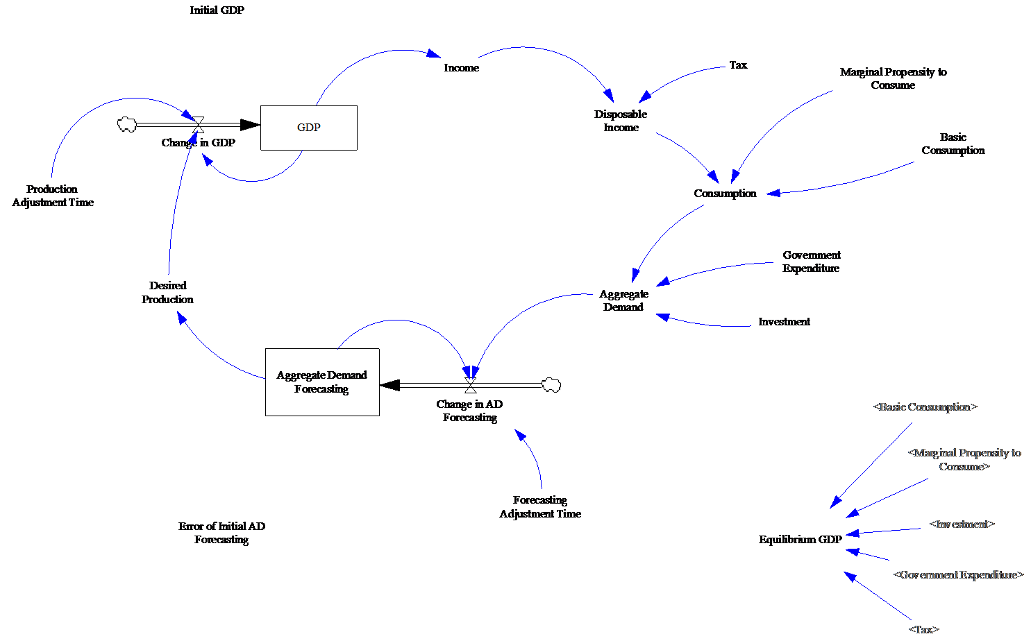
Figure 1 System Dynamics Keynesian Model

 

Description of Keynesian Model variables

In order to create the Keynesian system dynamic model of GDP (Figure 1), Yamaguchi (2015) used a simple Keynesian macroeconomic model to generate the aggregate demand equilibrium, which assumptions are described in this section. First, it is described the main equations that make part of the Keynesian macroeconomic model (Table 1).

Y = AD (Determination of GDP)	(1)
AD = C + I + G (Aggregate Demand)	(2)
C = C0 + cYd (Consumption Decisions)	(3)
Yd = Y – T – δK (Disposable Income)	(4)
T = T* (Tax Revenues)	(5)
I = I* (Investment Decisions)	(6)
G = G* (Government Expenditures)	(7)
dK/dt = I – δK (Net Capital Accumulation)	(8)
Yfull = F(K, L) (Production Function)	(9)
Yfull = Y (Equilibrium Condition)	(10)
dP/dt = (AD / P – Yfull)	(11)

Table 1 Equations to compose the Keynesian model

Yamaguchi argues that considering the neoclassical view that supply creates its own demand in the long run, he pointed out equation (1) was redundant. Due its assumption he added a new equation (11), which takes into account the price mechanism which adjusts discrepancies between Y_full and AD. The author call the equilibrium attained as neoclassical long-run equilibrium.

After this consideration, Yamaguchi points out according a Keynesian view GDP is determined by the aggregate demand in the short-run and in this sense, the equation (10) becomes redundant. According to Yamaguchi, the level of GDP is nothing but equal to the level of aggregate demand and needs not be the same as the amount of output produced by the economy’s production function (9).

Consequently, Yamaguchi argues that contrary to neoclassical view, the economy has no autonomous mechanism to attain an equilibrium in which output produced by the equation (9) is equal to the aggregate demand. Yamaguchi mentions this is because price is regarded as sticky in the short-run, and cannot play a role to adjust a discrepancy between aggregate supply of output and aggregate demand; but, according to Keynesian economists such a neoclassical long-run equilibrium could only be attained in the short run through changes in aggregate demand made possible by monetary and fiscal policies.

Considering these views Yamaguchi creates a synthesis model to deal with the mentioned controversies between neoclassical and Keynesian schools using a system dynamic approach. According to Yamaguchi, this is possible because, from a system dynamics point of view, macro economy is nothing but a system and different views on the behavior of the system can be explained as structural differences of the same system.

Based on the previous arguments, a new macroeconomic system was created in which a structure incorporates a bicurrency system. The next step adopted by Yamaguchi was to create a Keynesian adjustment process from which it is possible to have the Keynesian system dynamic model of GDP.

Keynesian adjustment process

Yamaguchi created a Keynesian adjustment process using the equations (1) to (9), with 9 unknown variables Y, AD, C, I, G, Y_d, T, K, Y_full with 7 exogenously determined parameters (C₀, c, T*, I*, δ, L).

According Yamaguchi a level of GDP that holds Y = AD is obtained in terms of the following equation:

Y* = (C₀– cT* + I* + G*) / (1 – c)                   (12)

Where Y* is the Keynesian equilibrium GDP.

Assigning some numerical values to these parameters[3]:

(C₀, c, I*, G*, T*) = (70, 0.6, 20, 10, 10)

Used for Y* = 235. Yamaguchi questions; how can such a Keynesian equilibrium GDP be attained if aggregate supply and aggregate demand are not equal initially? He answers this taking into account the Keynesian assumption that aggregate supply is determined by the size of aggregate demand. He illustrates this point of view through Figure 2 how an initial GDP of Y₀ continues to increase until it catches up with the aggregate demand, and eventually attains a Keynesian equilibrium Y*.

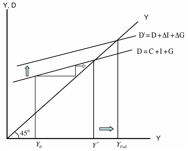
Figure 2 Keynesian determination of GDP

Observing the Figure 2, Yamaguchi pointed out there is no guarantee that the Keynesian equilibrium GDP of Y* is equal to Y_full from equation (9). He mentions when it is less than maximum output level, capital stock in under-utilized and some workers are unemployed; that is, the economy is in a recession. The author concludes, the Keynesian aggregate demand equilibrium is no longer equilibrium in the sense that capital and labor are fully utilized.

Yamaguchi uses the Keynesian arguments that the underutilization is caused by deficiencies of effective demand, and to gain full capacity and full employment equilibrium, additional effective demand has to be created by increasing investment and government expenditures, or decreasing taxes. He states the amount of new effective demand is given by the Keynesian multiplier process, which is derived from equation (12). Thus, the multipliers for I, G and T are calculated as follows:

         (13)

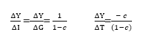
In order to simulate dynamically two points of equilibria for two different levels of aggregate demand, Yamaguchi argues the equation (1) has to be replaced with the following differential equation:

dY/dt = (AD – Y) / AT                        (14)

Where AT is an adjustment time. He states that in system dynamics this process is known as balancing feedback or goal seeking dynamics in which aggregate demand plays a role of goal and GDP tries to catch up with it. In system dynamics the equation (14) is represented by the following figure:

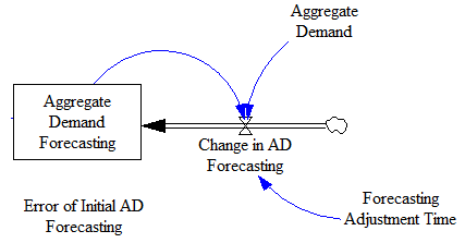
Figure 3 System dynamic representation of equation 14

The complete Keynesian system dynamic model of GDP without parallel currency is shown in Figure 1. The complete description of this model is given in the next section.

Description of the Keynesian system dynamics model of GDP

The equation for each component of Keynesian system dynamics model of GDP (Figure 4) is presented, as well as, values for some variables.

Name	Equation	Units
Income	= GDP	Dollar/Year
Disposable Income	= Income – Tax	Dollar/Year
Tax	= 10	Dollar/Year
Consumption	= Basic Consumption + (Marginal Propensity to Consume * Disposable Income)	Dollar/Year
Marginal Propensity to Consume	= 0.6	Dmnl
Basic Consumption	= 70	Dollar/Year
Government Expenditure	= 10	Dollar/Year
Investment	= 20	Dollar/Year
Aggregate Demand (AD)	= Consumption + Gov. Expenditure + Investment	Dollar/Year
Equilibrium GDP	= (Basic Consumption – (Marginal Propensity to Consume * Tax) + Investment + Government Expenditure) / (1 – Marginal Propensity to Consume)	Dollar/Year
Change in AD Forecasting	= (Aggregate Demand – AD Forecasting) / Forecasting Adjustment Time	Dollar/Year
Forecasting Adjustment Time	= 1	Year
AD Forecasting Initial Value	= Change in AD Forecasting = Equilibrium GDP * Error of Initial AD Forecasting	Dollar/Year Dollar/Year
Error of Initial AD Forecasting	= 0.8	Dmnl
Desired Production	= Aggregate Demand Forecasting	Dollar/Year
GDP Initial Value	= Change in GDP = Initial GDP	Dollar/Year Dollar/Year
Initial GDP	= 0	Dollar/Year
Change in GDP	= (Desired Production – GDP) / Production Adjustment Time	Dollar / Year Year
Production Adjustment Time	= 1	Year

Table 2 Description of the Keynesian SD model components

Three tests were done using the Keynesian system dynamic model of GDP. The time horizon was 20 years. Time step is yearly. The objectives of each test were to observe the GDP value, as well as, aggregate demand and Keynesian equilibrium model in three hypothetical situations: (1) there is no recession (test 1); (2) there is a recession caused by decrease in the marginal propensity to consume and where there is not government intervention; (3) there is a recession caused by reduction in the marginal propensity to consume but the government intervenes increasing its expenditure level.

All tests used the data from Table 2, i.e., with some variations. For example, in test 2 and 3, the marginal propensity to consume decrease from 0.6 to 0.3 during the years 11 to 14, increasing again to 0.6 from time 15 to 20.

In test 3, the government expenditure increase from 10 to 60 during the years 11 to 14, decreasing to 10 from time 15 to 20. The results from this test are shown in Table 3.

Test	Initial GDP	C	G	I	T	c	Y*	Y*rec	ADt=10	ADt=15	ADt=20	Yt=10	Yt=15	Yt=20
1	0	70	10	20	10	0.6	235	0	228.6	233	234.4	224.9	231.7	234
2	0	70	10	20	10	Table 3A	235	138	225.8	188.7	217	219.7	158	204
3	0	70	Table 3B	20	10	Table 3A	235	210	225.8	222	230	219.7	213	226.7

Table 3 Results of the tests using the Keynesian system dynamic model without parallel currency

C = Basic consumption; G = Government Expenditure; I = Investment; T = Tax; c = marginal propensity to consume

Y* = Keynesian equilibrium GDP; Y*rec = Keynesian equilibrium GDP during recession period (years 11 up to 14)

AD_t = Aggregate Demand at Year t; Y_t = GDP at Year t;

Table 3a – Marginal propensity to consume (c) values for tests 2 and 3			Table 3b – Government expenditures (G) values for tests 2 and 3
TIME	c		TIME	G
1 to 10	0.6		1 TO 10	10
11 to 14	0.3		11 TO 14	60
15 to 20	0.6		15 TO 20	10

Figure 4 shows the evolution of the Keynesian equilibrium GDP, aggregate demand and GDP for test 1. As is expected both the aggregate demand and GDP converge to the Keynesian equilibrium GDP along the time. This test represents an economy without economic shock, i.e., without economic recession.

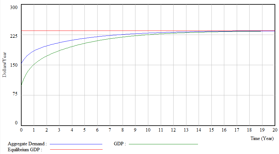
Figure 4 Evolution of the Keynesian equilibrium GDP, aggregate demand and GDP in test 1

Figure 5 represent the evolution of the Keynesian equilibrium GDP, aggregate demand and GDP for test 2. A reduction of the marginal propensity to consume from 0.6 to 0.3 during the time interval 11 to 14 years, caused drastic reduction in the three mentioned variables. It is important to note in this test the government expenditure was equal 10 during all simulation time. The marginal propensity to consume increases from 0.3 to 0.6 at time 15 to 20 all variables increase in different levels. Both the aggregate demand and GDP values at time 20 are lower than Keynesian equilibrium GDP. This is expected once the government did not increase its expenditure level.

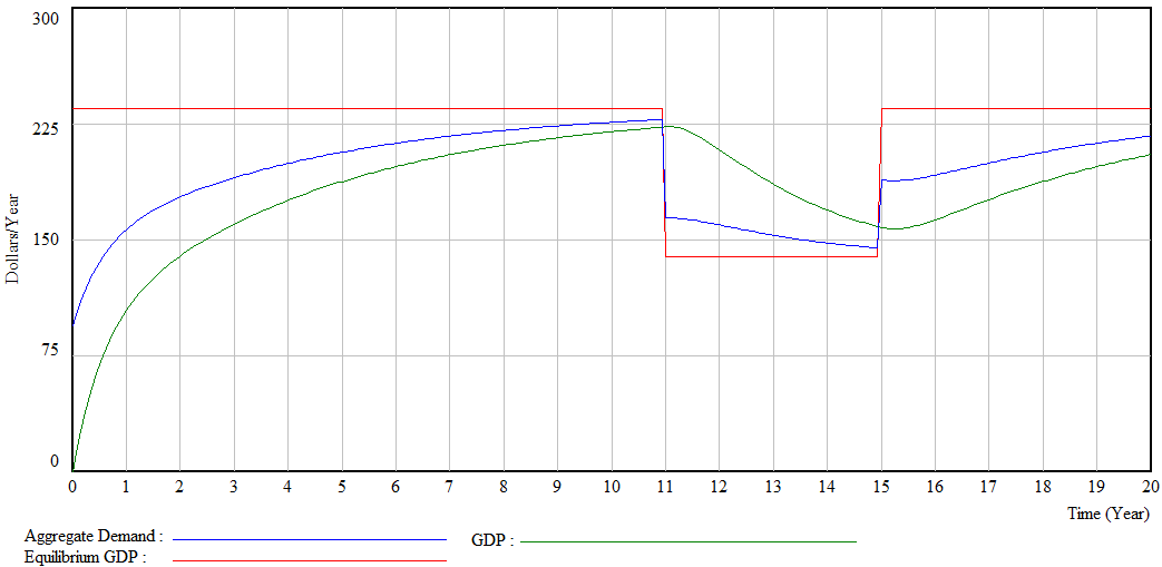
Figure 5 Evolution of Keynesian equilibrium GDP, aggregate demand and GDP for test 2

Figure 9 shows the evolution of the Keynesian equilibrium GDP, aggregate demand and GDP for test 3. As already mentioned, the difference between test 2 and test 3 is in the last one the government increased its expenditures during the recession period (between years 11 to 14) (Table 3b). In other words, its level of indebtedness increased during the recession period from 10 to 80.

As result of the government expenditures both aggregate demand and GDP values did not decrease during the recession period (Table 3).

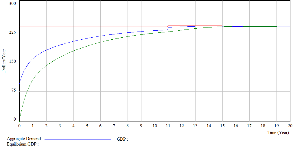
Figure 6 Evolution of Keynesian equilibrium GDP, aggregate demand and GDP for test 3

The results from tests 2 and 3 are expected according Keynesian theory. The advantage of simulating macroeconomic system using system dynamics is the flexibility to test new macroeconomic structures, such as, incorporating a parallel currency into the economy and assess its impact over the system along time (see next section). It worth mention that simulating a macroeconomic system allows the research to visualize the interactions of the variables along time and check its theoretical assumptions and hypothesis.

The next section describes the bicurrency system dynamics model of GDP.

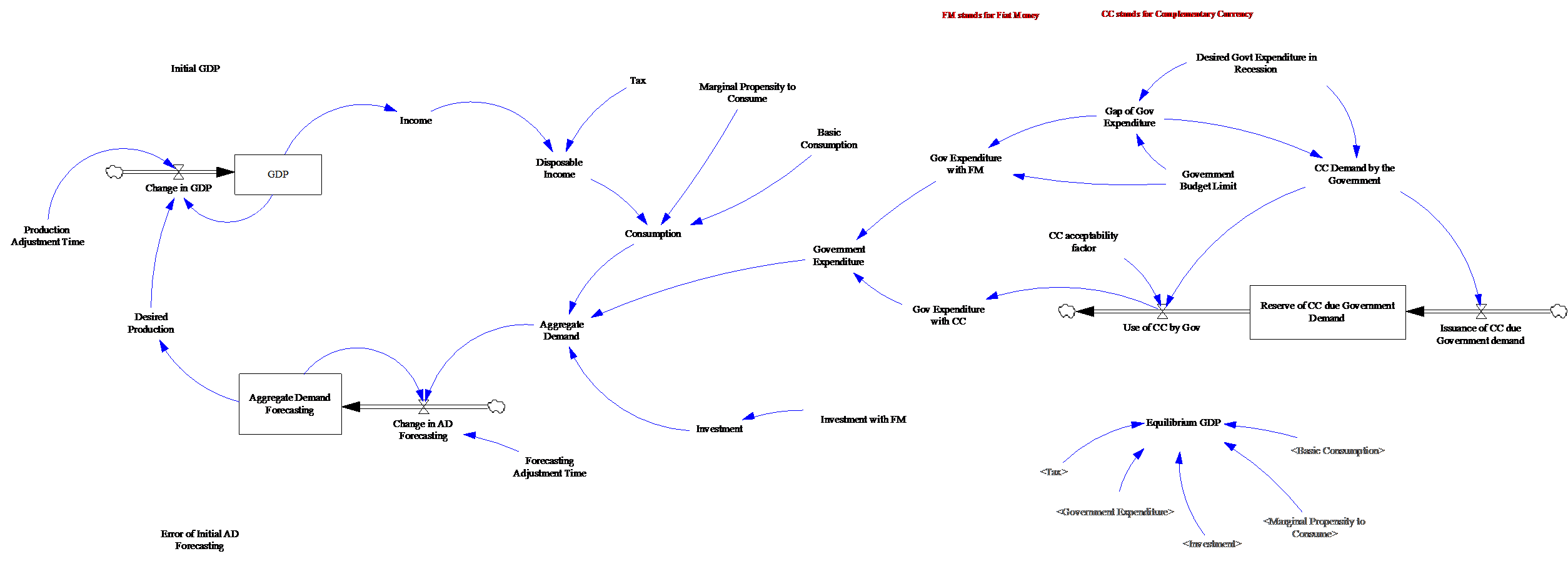
Figure 7 System Dynamics Bicurrency Model

Description of Bicurrency System Dynamics model of GDP

In the bicurrency system dynamic model of GDP the two government sources of money are represented, respectively, by “Government Expenditure with Fiat Money (Gov Expenditure with FM)” and “Government Expenditure with Complementary Currency (Gov Expenditure with CC)”. Details regarding the equations of the bicurrency model are shown in Table 3.

An auxiliary variable called “Government Budget Limit” was introduced to represent the yearly available government budget. In this model the government is not allowed to spend more than its yearly budget limit.

The variable Desired Government Expenditure in Recession was introduced to represent the amount of extra government expenditures that would be incurred in order to recover the economy during a recession period. The variable is a goal that can or not be attended.

In this model, it is assumed the government cannot exceed the budget limit during recession periods. Despite this fact, the government can issue complementary currency in order to finance the necessary activities to recover the economy during a recession period.

The demand of complementary currency by the government is given by the variable CC Demand by the Government which is calculated taken into account the “Gap of Government Expenditure (Gap of Gov Expenditure)”.  See Table 3 for details of the equation.

The government only will demand complementary currency during recession periods in order to expend it to recover the economic growth.

The value of CC Demand by the Government will be used by both input and output flow variables named, respectively, Issuance of CC due Government demand and Use of CC by Gov. See Table 3.

The input flow Issuance of CC due Government demand represents the issuance of the CC. The output flow Use of CC by Gov represents the expenditure of CC by the government. The variable CC acceptability factor means the level of acceptance of the complementary currency (CC) in the macroeconomic system. A value of 1 means total acceptance, the currency can be accepted partly so the range varies from 0 to 1.

The stock variable Reserve of CC by Government Demand is given by the difference between the input and output flows (Table 3).

The Reserve of CC Gov Demand will be greater than zero only if all issued complementary currency is not utilized by the government. This means, if the CC acceptability factor is less than 1.

The variable Gov Expenditure with CC represents the amount of Complementary currency used by the government during recession periods. Its value is equal to the output flow Use of CC by Gov.

Name	Equation	Units
Income	= GDP	Dollar/Year
Disposable Income	= Income – Tax	Dollar/Year
Tax	= 10	Dollar/Year
Consumption	= Basic Consumption + (Marginal Propensity to Consume * Disposable Income)	Dollar/Year
Marginal Propensity to Consume	= 0.6	Dmnl
Basic Consumption	= 70	Dollar/Year
Government Expenditure	= Government Expenditure with Fiat Money (FM) + Government Expenditure with Complementary Currency (CC)	Dollar/Year
		CC/Year
Gov Expenditure with Fiat Money	= IF THEN ELSE (Gap of Gov Expenditure > 0, Gap of Gov Expenditure, Government Budget Limit)	Dollar/Year
Government Budget Limit	= 10	Dollar/Year
Gap of Gov Expenditure	= IF THEN ELSE (Desired Gov Expenditure in Recession > Gov Budget Limit, (Gov Budget Limit – Gov Expenditure in Recession), Gov Budget Limit)	Dollar/Year
Desired Gov Expenditure in Recession	= 0	Dollar/Year
Complementary Currency (CC) Demand by the Government	= IF THEN ELSE (Gap of Gov Expenditure < 0, Desired Gov Expenditure in Recession, 0)	Dollar/Year
Issuance of CC due Gov Demand	= CC Demand by the Government	CC/Year
Reserve of CC due Gov Demand	= Issuance of CC due Gov Demand – Use of CC by Government	CC/Year
Use of CC by Government	= CC Demand by the Government * CC acceptability factor	CC/Year
CC acceptability factor	= 1	Dmnl
Gov Expenditure with CC	= Use of CC by Government	CC/Year
Investment	= 20	Dollar/Year
Aggregate Demand (AD)	= Consumption + Gov. Expenditure + Investment	Dollar/Year
Equilibrium GDP	= (Basic Consumption – (Marginal Propensity to Consume * Tax) + Investment + Government Expenditure) / (1 – Marginal Propensity to Consume)	Dollar/Year
Change in AD Forecasting	= (Aggregate Demand – AD Forecasting) / Forecasting Adjustment Time	Dollar/Year/Year
Forecasting Adjustment Time	= 1	Year
AD Forecasting	= Change in AD Forecasting	Dollar/Year
Initial Value	= Equilibrium GDP * Error of Initial AD Forecasting	Dollar/Year

Table 4 Description of the parallel currency SD model components

Two tests were done to assess the bicurrency model (Table 4). The values of test 1 are equal to the test 1 from Table 3. The objective of this test was to verify the behaviour of the model without recession period.

Test	Initial GDP	C	G	I	T	c	Y*	Y*rec	ADt=10	ADt=15	ADt=20	Yt=10	Yt=15	Yt=20
1	0	70	10	20	10	0.6	235	235	225.8	232	234	219.7	230	233.4
2	0	70	Table 5B	20	10	Table 5A	235	238	225.8	235	235	219.7	235	235

Table 5 Results of the tests using the system dynamic model with parallel currency

C = Basic consumption; G = Government Expenditure; I = Investment; T = Tax; c = marginal propensity to consume

Y* = Keynesian equilibrium GDP; Y*rec = Keynesian equilibrium GDP during recession period (years 11 up to 14)

AD_t = Aggregate Demand at Year t; Y_t = GDP at Year t;

Table 5a – Marginal propensity to consume (c) values for test2			Table 5b – Government expenditures (G) values for test 2 using Fiat Money (G_FM) and Complementary Currency (G_CC)
Time	c		TIME	G_FM	G_CC
1 to 10	0.6		1 TO 10	10	0
11 to 14	0.3		11 TO 14	10	70
15 to 20	0.6		15 TO 20	10	0

Figure 8 shows the evolution of aggregate demand, Keynesian equilibrium and GDP for test 2.

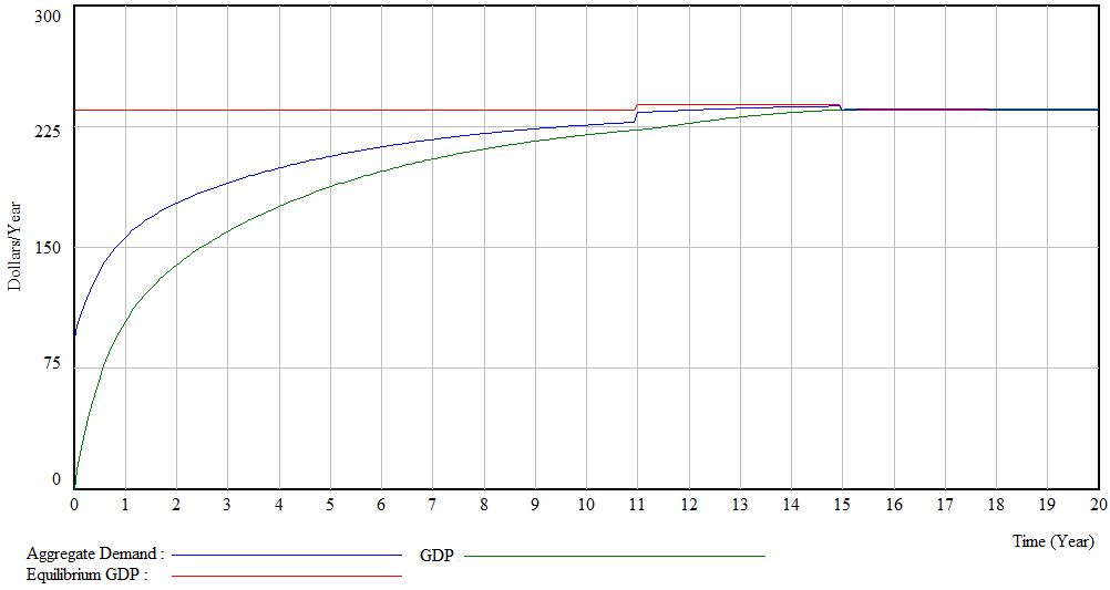
Figure 8 – Evolution of the aggregate demand, Keynesian equilibrium and GDP for test 2

The test 2 results show that the government intervention avoided the reduction in GDP and aggregate demand without the necessity to increase its level of indebtedness with fiat money. In this model the issuance of complementary currency does not increase the level of indebtedness and at the same time help the macroeconomic system becomes more resilient even when economic shocks occur, such as the reduction of the marginal propensity to consume.

Conclusion

This study sought to answer the question as to whether parallel currencies reduce the impact of credit shocks within an economy. The findings have shown that indeed, parallel currencies play a pivotal role in reducing the impact of credit shocks and sustaining economies during periods of financial crises. These currencies assist governments by providing an alternative means of financing expenditures during times of recession, other than through the fiat money thereby reducing the governments’ level of indebtedness

The literature review tells success stories on the application of parallel currencies during economic recessions to stimulate the economy and reduce unemployment levels. Notable cases highlighted include the Wörgl case study, the Brixton Pound and the WIR Franc among others. Similarly, the findings support the initial hypotheses that the incorporation of a parallel currency in a macroeconomic system helps the government to overcome economic recession avoiding increasing its level of indebtedness with fiat money. The findings also prove that it is possible to test the impact of parallel currencies through the simulation of a hypothetical macroeconomic system using system dynamics methodology.

The study underscores the fact that a closed economy operating a bi-currency system can overcome the negative consequences of credit shocks by expanding government expenditure using the parallel currency. Therefore, authorities would not have to adopt expansionary monetary policies on fiat money to deal with high unemployment. Parallel currency will reduce the governments’ indebtedness during a recession.

Discussion

The history shows us some study cases; Wörgl case study, Brixton pound and WIR Bank. Where the use of parallel currency helps the economy to be more resilient and avoid negative consequences of the economic recessions, such as, unemployment. The result of this macroeconomic bicurrency system dynamic model shows us that the insertion of a parallel currency avoids the reduction of aggregate demand and GDP, once the government spend without getting indebtedness.

This model needs improvement, such as, incorporate other sectors that compose a macroeconomic system, as well as, incorporate the foreign relationship between countries. This model can be improved by defining the consumers within an economy; consumer savings, consumer consumption, consumer investment. The model could be improved by adding a central bank, who is responsible for giving out government securities and money supply.

We need to add the following things to the discussion:

The acceptability of the complementary currency is quite important.

This will mean that if the habitants doesn’t accept the currency or even partly is accepted, it will cause problems. Also look for the legal evidence about this within Europe. It main discussion point is of this model and parallel currencies can be used in the real world. This is the part to add the real world perspective. Is it possible to introduce this into Europe. Can Greece legally add another currency while everybody within the EU agreed to use the Euro.

Apparently this model works, but which bumps can we expect when we do introduce this parallel currency. Do consumer use this currency to spend and how will they collect this currency. Explain the real world perspective in this part. This part will break or make the master thesis.

We also could hit some legal problems. In example when Greece wants to introduce a national parallel currency, there could be a law against this from the European Union. Countries within the Euro can’t introduce a national parallel currency. It is wise to find a source with this.

We should also add that this is concerning a closed economy. An addition towards the model would add the exports and imports of the country. This need to include chapter 6 of Blanchard; here is explained what the added value of an open economy is.

Openness of an economy

Step 1. Explain what an open economy is. The difference of the IS-LM model open economy and the IS-LM model closed economy. The IS-LM model closed economy is used in the thesis to preform test with a parallel currency.

Step 2. Valid arguments why exports and import should be added to the model

The import and export would be effected. A country with a parallel currency tend to invest more in their own economy. National currency is relative sarce so it would be easier to use a parallel currency to buy goods and services.

Maybe we could explain the exchange rate between the national currency and foreign currency. What will happen to this exchange rate? In order to explain what will happen to this, the theory behind it should been explained first.

The foreign exchange rate should be explain as the exchange rate is the only part the differs from the closed economy IS-LM model.

Arguments would be that for the domestic country it would be more attractive to buy local. This would affect the market in a way that the domestic country has a decrease in imports. However this is only theory based and could be added in the system dynamic model.

For more academic help please check a wide range of services our Economics Writing Help team offers:
– Economics Assignment Writing Services
– Economics Essay Writing Services
– Economics Dissertation Writing Services
– Buy An Economics Research Paper

Here you can check some of our dissertation services:
– Dissertation Writing Services
– Write My Dissertation
– Buy Dissertation Online
– Dissertation Editing Services
– Custom Dissertation Writing Help Service
– Dissertation Proposal Services
– Dissertation Literature Review Writing
– Dissertation Consultation Services
– Dissertation Survey Help